Contents
Concepts
Statistical assessment of reliability and validity
Assessment of the reliability and validity of a measurement method is a multi-faceted undertaking, requiring a range of statistical approaches. Reliability and validity are quantified in relation to the intended practical requirements of the measurement tool [1]. Validity and reliability can be assessed in either relative or absolute terms, as described in Table C.7.1. Statistical approaches used to assess both the association (relative) or agreement (absolute) between two sets of data in studies of reliability or validity are described in the following sections.
Table C.7.1 Relative and absolute forms of reliability and validity.
| Relative | Absolute | |
|---|---|---|
| Reliability | The degree to which individuals maintain their position in a sample with replicate measurements using the same method | The agreement between replicate measures of the same phenomenon using the same method and units |
| Validity | The degree to which two methods, irrespective of units, rank individuals in the same order | The agreement between two methods measuring the same phenomenon with the same units |
Correlation coefficients describe the association between two variables, irrespective of their measurement units. The two variables can come from replicate measures using the same method (reliability), or from different methods (validity). The correlation coefficient is a dimensionless numerical quantity in the range from -1 (perfect negative correlation) to +1 (perfect positive correlation), with 0 representing no correlation. It can be used to assess relative reliability or validity; the closer the correlation coefficient is to +1, the higher the relative reliability or validity. However, a high correlation does not necessarily imply high absolute reliability or validity.
A statistical test can be performed of the null hypothesis that the true correlation is zero but this is less useful for assessing reliability and validity. It is to be expected that two measures of the same phenomenon are related to some degree. Even small numerical values of the correlation coefficient could appear to be “statistically significant” (e.g. p<0.05) if the sample size is large. In addition, two methods may also have correlated error (e.g. two self-report instruments) which would inflate the correlation between them. Correlation coefficients and their significance should therefore be interpreted with caution in the context of reliability and validity.
Examples of correlation coefficients used to assess reliability and validity include:
- Pearson correlation coefficient, which describes the direction and strength of a linear association between two continuous variables. Pearson’s r can be affected by sample homogeneity which makes distinguishing between individuals more difficult. High correlation does not rule out unacceptable measurement error.
- Spearman rank correlation coefficient (commonly denoted Spearman's rho) which describes the direction and strength of a monotonic association between the rankings of two continuous variables. Two variables have a monotonic association if either
(i) as the values of one variable increase, so do the values of the other variable, or (ii) as the values of one variable increase, the values of the other variable decrease. It is possible for the association between two variables to be monotonic but not linear. While this method typically yields lower values than the Pearson correlation coefficient for normally distributed variables, Spearman's rank correlation is less affected by outliers. - Kendall rank correlation coefficient (commonly denoted Kendall's tau) is an alternative to the Spearman rank correlation coefficient, specifically used for variables measured on an ordinary rather than continuous scale.
- Intraclass correlation (described in more detail below)
It is possible that measurement methods are strongly correlated but have very little absolute agreement. Correlation coefficients are not able to detect systematic bias [2]. However, absolute validity or reliability may not be required depending on the research question. One example would be when only accurate ranking of individuals within a population is required, such as in a study examining whether a measured lifestyle exposure is or is not associated with a disease [3]. In this type of study, a method with high relative reliability and validity as demonstrated by a high correlation coefficient may be suitable; if the purpose of the study were to determine the exact dose-response relationship, relative validity of the method used to measure the exposure would not be sufficient.
Unlike the correlation coefficients discussed above, which describe the association between two variables, the ICC describes the extent of agreement [4]. The variables can either be from replicate measures using the same method (reliability), or from two (or more) methods measuring the same phenomenon (validity). Since the ICC describes agreement between variables, it is typically used to determine absolute reliability or validity.
An advantage of the ICC is that it can be used to assess agreement between more than two sets of measurement (i.e. from three different observers of the same phenomenon, or multiple days of measurement). The ICC can be calculated in different ways which yield different estimates of reliability or validity. ICC values closer to 1 represent greater reliability or validity.
The ICC can be affected by sample homogeneity; if a study sample is highly homogeneous, it is more difficult to distinguish between individuals and the ICC would be comparatively lower than if the same measurements were compared in a more heterogeneous sample.
Linear regression is a method to model the linear association between two variables. When used to assess reliability, the two variables come from replicate measures of the same quantity using the same method. When used to assess validity, the variables are from two different methods measuring the same quantity.
Linear regression using least squares is the most common method but other types of regression exist [5]. Regression models used to assess validity may have multiple independent input variables. Similarly, non-linear relationships can be modeled using non-linear transformations of one or more of the included variables in a regression model.
General principle
Values of two replicate measures (reliability) or from two methods (validity) can be plotted in a scatterplot: one variable (the independent or predictor variable) on the x-axis against the other variable (the dependent variable) on the y-axis. Figure C.7.1 shows examples of scatterplots with the best fitting straight line obtained from linear regression as a dashed line in each plot. The equation of the best fitting regression line is shown on the form y = mx + c; the line of unity (y=x) is also included as a solid line. The slope (m) represents the expected increase in y if x were to increase by one unit, the intercept (c) is the expected y value when x = 0. For absolute reliability and validity, the expectation for perfect agreement is a slope of 1 and an intercept of 0 [6].
A common statistic accompanying a regression model is the coefficient of determination, or R2. This provides a measure of the proportion of the variability in the dependent variable that can be explained by variability in the independent variable(s). Conversely, 1 - R2 is the proportion that remains unexplained by the regression model.
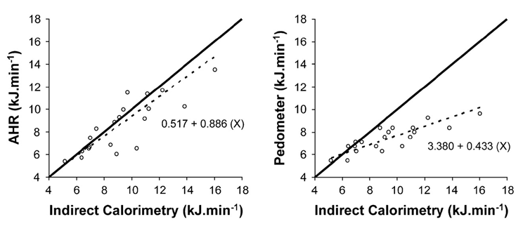
Figure C.7.1 Example of scatterplots and regression equations. As a reference, energy expenditure from indirect calorimetry is plotted on x-axis. On the left, energy expenditure estimated from a combined accelerometer and heart rate (AHR) is presented. On the right, energy expenditure estimated from a pedometer is presented. Source: Thompson et al, 2006 [7].
Systematic error
Suppose that validity of the variable on y-axis is of interest. Its systematic error in reference to the other on x-axis can be described using the intercept and slope of the regression line:
- The intercept ‘c’ provides a measure of the fixed systematic error between the two variables, i.e. one method provides values that are different to those from the other by a fixed amount. A value of 0 for c indicates no fixed error. Confidence intervals (e.g. 95%) can be used to examine whether c ≠ 0 and thus determine whether fixed error is statistically significant.
- The slope, m, provides a measure of the proportional error between the two variables, i.e. one method provides data that are different to those from the other by an amount that is proportional to the level of the measurement. A value of 1 for m indicates no proportional error. Confidence intervals (e.g. 95%) can be used to examine whether m ≠ 1 and thus determine whether proportional error is present.
Random error
Random error inherently exists in any measurements. The influence of random errors on the regression estimates vary according to whether the error is present in the variable on y-axis or the other on x-axis. If the random error were present in the variable on y-axis, estimates of the slope and intercept would become more imprecise, but estimates themselves would be unbiased. By contrast, if the error is present in the variable on x-axis, the slope would be attenuated or ‘diluted’ toward the null.
Uncertainty in a regression model
Uncertainty in parameter estimates from a regression is an important consideration [8]. Uncertainty increases when:
- The data are not evenly distributed over the measurement range
- The number of data points is low
- The data points are not independent of each other
- The relationship between the two variables is not linear
- The magnitude of variability relative to the data range is high
Errors of one method against another (reference) can be described by the root mean square error (RMSE), i.e. the square-root of the mean squared differences between methods. It is also a commonly used statistical measure of goodness-of-fit in regression. This statistic amplifies and severely punishes larger errors. A lower RMSE indicates greater agreement at individual level.
The agreement between two continuous variables (A and B) in the same units from replicated measures using the same method (absolute reliability), or from different methods (absolute validity), can be assessed using Bland-Altman plots [9]. The difference between each pair of values (A-B) on the Y axis is plotted against the mean of each pair ((A+B)/2) on the X axis (Figure C.7.2). Alternatively, the difference between each pair of values can be plotted against just one of the variables (a criterion method) on the X-axis. The purpose is the same; to examine differences between measurements across the range of (true) underlying values of the quantity of interest.
Assessing reliability or validity in this way provides:
- Quantification of the difference between replicate measurements (reliability) or different methods (validity) rather than how related they are, meaning that systematic differences between methods can be detected (e.g. between a new method and a criterion method)
- Indication of whether the difference between values is related to the magnitude of the quantity of interest. In Figure C.7.2, the variability of the difference between two measures increases at higher levels of the quantity of interest (a phenomenon known as heteroscedasticity). Two methods may demonstrate good agreement at the low end of the scale but have poor agreement at the high end of the scale.
- The magnitude and direction (i.e. positive or negative) of systematic bias is represented by the mean of all differences between paired values (solid horizontal line in Figure C.7.2)
- Random error is estimated by the standard deviation of these differences (dashed horizontal lines at +/-2 standard deviations in Figure C.7.2)
 and the weighed record (WR). Solid line = mean difference or systematic bias; dashed lines = plus and minus two standard deviations.")
Figure C.7.2 Agreement analysis for vitamin E intake estimated with semi-quantitative food frequency questionnaire (SFFQ) and the weighed record (WR). Solid line = mean difference or systematic bias; dashed lines = plus and minus two standard deviations.
Source: Andersen et al. (2004) [10].
Cohen’s kappa, K, is a measure of agreement between two categorical variables; it is commonly used to measure inter-rater reliability [8], but can also be used to compare different methods of categorical assessment (e.g. validation of a new classification method). It improves upon percent agreement between scores by taking into consideration the agreement we would expect due to chance (i.e. if the two measurements were unrelated).
It is calculated as the amount by which agreement exceeds chance, divided by the maximum possible amount by which agreement could exceed chance. A value of K closer to 1 indicates perfect agreement, whereas 0 represents the amount of agreement that can be expected due to chance.
Other kappa statistics include:
- Fleiss kappa, which is an adaptation of Cohen’s kappa for more than two sets of observations.
- Weighted kappa, which is used when a variable has multiple ordered categories. This technique assigns different weights to the degree of disagreement, for example for a 5-category ordinal variable the disagreement between categories 1 and 5 is greater than the disagreement between categories 1 and 2.
A receiver operating characteristic curve can be used to optimise a binary classification (two categories) from a continuous variable. A ROC curve illustrates the effect of varying the discriminatory threshold for the classification by plotting the true positive rate (sensitivity) against the false positive rate (1 - specificity).
The area under the curve (AUC) is a measure of the ability of the continuous variable to inform the classification; an AUC of 1 means perfect classification and an AUC of 0.5 is equivalent to flipping a coin, thus indicating the lower boundary of actual information above chance [12].
- Atkinson G, Nevill AM. Statistical methods for assessing measurement error (reliability) in variables relevant to sports medicine. Sports Medicine (Auckland, N.Z.). 1998;26:217-38
- Schmidt ME, Steindorf K. Statistical methods for the validation of questionnaires--discrepancy between theory and practice. Methods of Information in Medicine. 2006;45:409-13
- Masson LF, McNeill G, Tomany JO, Simpson JA, Peace HS, Wei L, Grubb DA, Bolton-Smith C. Statistical approaches for assessing the relative validity of a food-frequency questionnaire: use of correlation coefficients and the kappa statistic. Public Health Nutrition. 2003;6:313-21
- Müller R, Büttner P. A critical discussion of intraclass correlation coefficients. Statistics in Medicine.1994;13:2465-76
- Ludbrook J. Linear regression analysis for comparing two measurers or methods of measurement: but which regression? Clinical and Experimental Pharmacology & Physiology. 2010;37:692-9
- Hopkins WG. Bias in Bland-Altman but not regression validity analyses. Sportscience. 2004;8:42-6.
- Thompson D, Batterham AM, Bock S, Robson C, Stokes K. Assessment of low-to-moderate intensity physical activity thermogenesis in young adults using synchronized heart rate and accelerometry with branched-equation modeling. The Journal of Nutrition. 2006;136:1037-42
- Twomey PJ, Kroll MH. How to use linear regression and correlation in quantitative method comparison studies. International Journal of Clinical Practice. 2008;62:529-38
- Bland JM, Altman DG. Statistical methods for assessing agreement between two methods of clinical measurement. Lancet (London, England).1986;1:307-10
- Andersen LF, Lande B, Trygg K, Hay G. Validation of a semi-quantitative food-frequency questionnaire used among 2-year-old Norwegian children. Public Health Nutr. 2004;7(6):757-64.
- McHugh ML. Interrater reliability: the kappa statistic. Biochemia Medica. 2012;22:276-82
- Hanley JA, McNeil BJ. The meaning and use of the area under a receiver operating characteristic (ROC) curve. Radiology. 1982;143:29-36

- The Toolkit
- About
- What's new
- Other resources
- Toolkit Team
- Contact
- Links to other toolkits
- Nutritools
- NCI/NIH Dietary Assessment Primer
- © 2026 MRC Epidemiology Unit
- Privacy policy and cookies
- Terms of Use