• Introduction
• Random error
• Systematic error
• Differential and non-differential errors
• Forms of bias
• References

All measures of diet, physical activity and anthropometry contain some degree of measurement error. Understanding the sources of this error is vital to help refine and develop the method, and strengthen the inferences that are made from the data. It is also important to understand that:

1. Measurement error and bias are different
2. Measurement error does not necessarily cause bias
3. Bias depends on the research question, i.e. how the measured quantity is used

The sources of measurement error fall into two categories:

1. Random error
2. Systematic error

These two types often co-exist. Scrutinising the sources and magnitude of both types of error is an important part of the research process, including deciding whether or not a method is appropriate for answering a particular research question.

Effect of random error on estimated values

1. Random errors cause the estimated values to deviate from the true value due to chance alone
2. They lead to measurements that are imprecise in an unpredictable way, resulting in less certain conclusions
3. Random error is assumed to cause predicted values to fluctuate above and below the true value by the same extent
4. This means that estimates of central tendency such as the mean or median are unaffected, but greater random error does increase the variability about the mean
5. Methods with less random error produce values which are closer together; this is known as the method’s precision

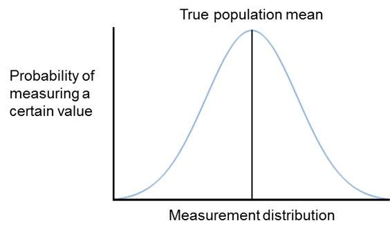
For example, a calibrated set of digital weighing scales may not show exactly the same reading on each measurement due to small fluctuations in posture and instrumentation. Measured values will be dispersed in a normal distribution around the true weight (Figure C.4.1). Methods with high random error will be more dispersed, methods with low random error less so. For both methods, with repeated measurement the true value can be estimated as the mean of the values from each. Estimates based on the mean from both methods may be similar, however we can be more certain about estimates given by the method with smaller random error.

Figure C.4.1 The normal distribution of measured values due to random errors. Note that the mean of the measured values approximates the true population mean.

Sources of random error

Random error can occur for a variety of reasons. These include:

1. Individual biological variation, e.g. biochemical measurement
2. Sampling error, e.g. subset of a larger population only selected
3. Measurement error, e.g. estimation of portion sizes in a dietary assessment

Examples of random error in diet, physical activity and anthropometric measurement include, but are not limited to, errors resulting from:

1. Inadequate or confused explanations from the investigators
2. Changes in behaviour due to the measurement procedure
3. Dietary coding errors
4. Participant error in estimating portion sizes
5. Limitations within a nutrient database
6. Improper calibration of instruments
7. Inconsistent placements of instruments on the body
8. Incorrect translations or coding of outcome data

If the error can be directly linked to specific factors, the error is not random, but systematic. For example, errors caused by inadequate recall may differ by specific personal traits, such as age – this would be a systematic error (see section below).

Controlling random error

Random error generally affects a method’s reliability. Random errors may be reduced or compensated for by:

1. Pilot work, particularly when designing new methods such as a new questionnaire
2. Increasing the number of measurements taken per participant
3. Increasing the sample size or the length of follow-up in a cohort study
4. Frequent calibration of instruments
5. Incorporating quality control and assurance in the assessment process:
1. Rigorous standard operating procedures
2. Manual of procedures
3. Standardised rigorous and consistent training of fieldworkers/interviewers undertaking assessments
4. Inter- and intra-observer reliability checks. An example of assessing this aspect for the measurement of waist circumference is provided in the table below.

Technical error of measurement (TEM)
Measurement error is caused by the interaction between the instrument, the technique, the observer taking the measurement and the characteristics of the participant.
The technical error of measurement (TEM) is an accuracy index. In anthropometry for example, it is the most common way to express error margin. It is the standard deviation between repeated measures, and it is a measure of error variability that carries the same measurement unit as the variable measured (e.g. cm for waist circumference). This is known as the absolute TEM. TEM can also be expressed as a percentage (known as relative TEM).

TEM = √ (∑D²) / 2N  

D is the difference between measurements
N the number of volunteers measured

TEM is used for the calculation of the intra-observer error – which is the variation of the repeated measurements of the same participant (or a group of participants) measured by the same observer; and for the calculation of between/inter-observer error – which is the variation of measurements performed by different observers on the same participant.

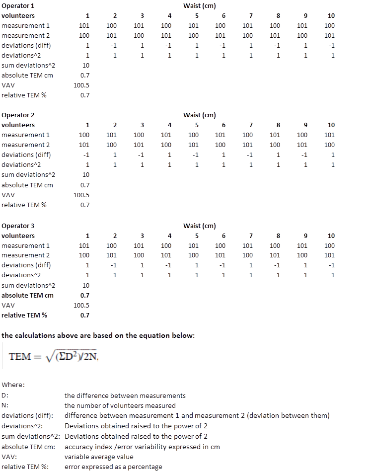
These calculations are typically carried out for quality control purposes during data collection and their evaluation is crucial for the observer to be able to improve the performance of the procedures through a training process. It is necessary for TEM to be reported in manuscripts on studies with repeated measures to analyse whether the observed differences are superior to TEM. Otherwise, the observed differences may not be attributed to exposure/intervention but to the TEM. The lower the TEM obtained, the better is the precision of the observer in performing the measurements. Typically, the expected TEM values that we observe in professional teams are between 0-0.2% for height and 1-2% for waist measurements. Its interpretation is that the differences between repeated measurements will be within ±2 the value of TEM two thirds of the time. TEM values for observers are considered adequate if they are within ±2 times the expert TEM (when 95% of the differences between replicate measurements are within ±2 TEM). Figure 4.2 displays an example of TEM calculation for 3 observers who did anthropometric measurements for 10 participants.

Figure C.4.2 Example of Intra-observer error calculation for the waist measurement based on 3 observers and 10 participants.

Effect of systematic error on predicted values

Systematic error causes deviation away from the true value in a particular direction (i.e. higher or lower, as shown by Figure C.4.3 below). Unlike random error (see section above), systematic error distorts the mean and median of the estimated values; it is therefore a measure of the absolute validity of a method. The validity page describes systematic error in the context of taking height measurements of participants wearing shoes. This causes deviation from the true body height in an upwards direction. While random error can be compensated for by increasing the number of measurements for an individual or the sample size, this systematic error would persist to the same extent, no matter how many replicate measurements were taken.

Systematic error does not always result in bias

If measurements of physical activity or water consumption were performed only in summer, those individuals’ levels over a year were likely to be overestimated because each exposure level is higher in summer than in winter. This is a systematic error due to insufficient sampling across seasons.

However, if the degree of the overestimation is consistent across individuals, the ranking of individuals by physical activity or water consumption level is unbiased, and associations with other characteristics would be unbiased. On the other hand, if the overestimation was proportional, say 10% higher in the summer, this would lead to slightly different associations since, for physical activity work, the most active individuals would have higher absolute systematic error than less active individuals. 

If researchers are primarily interested in relative levels, rather than estimating absolute levels of a key variable, systematic error is not always problematic. Ideally, this would be tested in a subset of a study to confirm that systematic error does not distort the ranking of individuals.

In research on population health, assessments of diet, physical activity and anthropometry are implemented in different population subgroups depending on the research question. These subgroups may be defined by: sex, age, socioeconomic status, lifestyle behaviours, risk factors for a disease, disease status, and the degrees of systematic and random errors may vary by those characteristics.

If error varies by one or more of those characteristics, the error is differential; and if not, the error is non-differential. For example:

1. Men and women may both over-report physical activity (systematic error), but this may be greater in males leading to a higher proportion being categorised as meeting guidelines (differential systematic error by sex)
2. Alternatively the misclassification can occur non-differentially, whereby the degree of misclassification is the same by group (i.e. men and women over-reporting physical activity to the same degree; non-differential systematic error by sex)

Wording can vary in the literature; terms such as homogeneity (non-differential) or heterogeneity (differential) in errors by subgroups are often used.

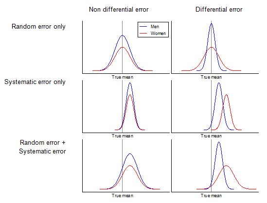
Different types of errors are visualised in Figure C.4.2, which illustrates:

1. If random error is present, variability is wide
2. If systematic error is present, mean estimate deviates from a true mean
3. If differential error is present, random error, systematic error, or both are different between men and women

Figure C.4.3 Display of random, systematic, differential, and non-differential errors with respect to men and women.

Bias is the term used to describe the cumulative effect of deviation of observations from truth which investigators wish to measure. In the example above, the poor calibration of the weighing scales was just one form of bias that distorted the weight data consistently upwards.

There are at least 50 forms of bias that occur in population health sciences and several different systems for classifying and subcategorising them. One of the simplest systems is to separate them into:

1. Information bias
2. Selection bias
3. Confounding

Further information regarding the categories and subcategories of bias can be found in the following article [1].

Information bias

Information bias is a result of errors introduced during data collection and is therefore the form of bias most applicable to the issue of measurement. These errors originate from:

1. Those measuring the variable, known as observer bias. For example, researcher knowledge of hypotheses and group allocations could influence the way information is collected and interpreted.
2. The tool being used for measurement, known as measurement bias. For example a malfunctioning gas analyser or poorly designed questionnaire.
3. Those being measured, known as respondent bias. This can take many forms, such as:
1. Social desirability bias, which can cause over- or under-reporting of certain behaviours, in order to appear favourable or avoid criticism
2. Recall bias, which occurs due to differences in the accuracy or completeness of recollections by study participants relating to prior events or experiences

These forms of bias can result from different forms of errors (e.g., mixture of differential and non-differential systematic and random errors)

Observer and respondent bias can be minimised by undertaking many different approaches: training observers, requesting participants not to change lifestyle during a study or behave differently when being monitored, and others as described above (see maximising reliability).

In a randomised controlled trial, participants and observers are ideally blinded to the intervention so that they do not behave differently. The same principles apply for measurement as administration of assessment is also a form of intervention.

Selection bias

Selection bias occurs when the study sample is systematically unrepresentative of the target population about which conclusions are to be drawn, resulting in data with insufficient external validity. The resulting data may therefore be flawed in its ability to answer any research questions about the target population, even if the study itself has a high level of internal validity. Selection bias can occur because of:

1. The way the study population (or subgroups) is defined
2. The inclusion or exclusion criteria
3. Study withdrawals/rate of follow up
4. Non-responders

Selection bias can often be reduced through careful study design, ensuring that no element of recruitment or data collection systematically favours one type of individual over another, as well as actively monitoring the characteristics of the sample population during the course of the study.

If selection bias is likely to exist by design, it is helpful to collect other information which makes it possible to estimate the likely size and direction of the bias in the results. For instance, it is possible to collect the demographic characteristics of non-responders, who can then be compared with the responders to determine whether they differ systematically by social status, education etc.

Confounding

Confounding does not result from measurement error and is not a measurement issue per se, but is an important epidemiological concept relating to study design, analysis and interpretation of data. Although confounding does not directly generally affect choice of method of assessment directly, it is important to ensure that potential confounding variables are measured using reliable and valid methods in order to reduce the effect of residual confounding. There are three criteria for confounding:

1. Variable has an independent association with the outcome of interest
2. Variable has an association with both the exposure and outcome
3. Variable is not on the causal pathway linking the exposure to the outcome

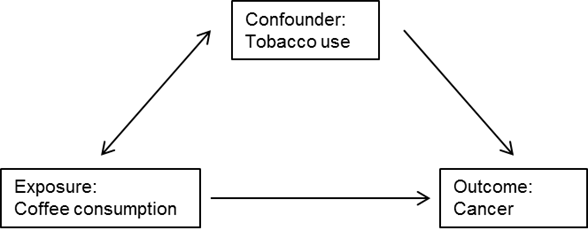
In typical epidemiological research on a lifestyle-disease association, confounding is explained with a graph, e.g. Figure C.4.4.

Figure C.4.4 Example of the relationships between an exposure, outcome and confounder.

In the above example, one of the assumptions is that smoking status is not on the causal pathway of the coffee-cancer relationship or, in other words, coffee consumption does not change smoking status. Confounding is controlled in the design of a study by randomisation, restriction or matching of participants, and during the analysis phase by stratification or statistical modelling.

1. Delgado-Rodríguez M, Llorca J, Bias. J Epidemiol Commun Health. 2004;58:635-41